What do avoided crossings sound like?

One interesting mathematical phenomenon I encounter regularly in my research¹ is that of avoided crossings. These emerge when, over the course of the evolution of a dynamical system, any two of its normal-mode frequencies become near-degenerate. If the two normal modes should be weakly coupled to each other in some fashion, then rather than actually becoming degenerate (and having their eigenfrequencies cross), the system responds in such a way that the actual normal modes exchange character smoothly between the two uncoupled modes; during this process the actual mode frequencies also interpolate smoothly between their uncoupled values.

I've made some sonifications of seismic data before for outreach purposes (and it sounds quite messy to the untrained ear), but I've been wondering lately what an idealised avoided crossing would sound like instead. In particular, would the human ear be able to distinguish between different strengths of coupling between the isolated components? I also haven't written a technical blog post in quite a while, and I thought this would be an interesting exercise. Here we go!

import numpy as np
import matplotlib.pyplot as plt

For this blog post I will be producing CD-quality PCM WAV files at a standard sampling rate of 44.1 kHz with 16 bits of dynamic range.

from scipy.io import wavfile
sampling = 44100 # Hz
duration = 5 # seconds

t = np.linspace(0, duration, duration * sampling, endpoint=False)

def raster(fname, f, norm=None):
    if norm is None:
        norm = np.max(np.abs(f))
    data = np.int16(np.maximum(-1, np.minimum(1, f / norm))
                    * 32767)
    wavfile.write(fname, sampling, data)

We first set up a test system of two pure tones. One of them will be middle A (440 Hz), and for the other we will do an exponential frequency sweep from the octave below it to the one above. If you have a time-dependent frequency $\omega(t)$, however, you can't just demand that your waveform be $\sin [\omega(t) t]$; instead, it has to be a chirp: $\sin \phi(t)$ such that ${\mathrm d \phi \over \mathrm d t} = \omega(t)$.

from scipy.integrate import cumtrapz

nu_A = 440 # Hz
pure_tone = np.sin(2 * np.pi * nu_A * t)

def chirp(nu, phase=0):
    assert len(nu) == len(t)
    φ = 2 * np.pi * cumtrapz(nu, t, initial=phase)
    return np.sin(φ)

nu_sweep = nu_A * np.power(2, -1 + 2 * t/duration)
sweep = chirp(nu_sweep)

We now have two “isolated” frequencies, $\nu_A$ and $\nu_\mathrm{sweep}(t)$. Given any two frequencies near resonance, we can describe an avoided crossing with two “coupled” frequencies

where the coupling strength $\alpha$ heuristically sets the minimum difference in frequency between the two resulting modes (i.e. it is zero for two completely decoupled modes).

# avoided crossings
from scipy.signal import stft
dashed = dict(ls='dashed', lw=1, c='gray')
for i in range(8):

    α = i**2

    nu_1 = (nu_A + nu_sweep) / 2 + np.sqrt((nu_A - nu_sweep)**2/4 + α**2)
    nu_2 = (nu_A + nu_sweep) / 2 - np.sqrt((nu_A - nu_sweep)**2/4 + α**2)

    signal = chirp(nu_1) + chirp(nu_2)
    raster(f"{i}.wav", signal, norm=2)

    ff, tt, Z = stft(signal, sampling, nperseg=sampling/10)
    plt.pcolormesh(tt, ff[1:] / nu_A, np.abs(Z[1:])**2, cmap='Blues')
    plt.plot(t, 1 + 0 * t, **dashed)
    plt.plot(t, nu_sweep / nu_A, **dashed)
    plt.gca().set_yscale('log', base=2)
    plt.ylim(1/2, 2)
    plt.ylabel(r"Frequency (vs. reference)")
    plt.xlabel(r"Time/s")
    plt.savefig(f"{i}.png", bbox_inches='tight', transparent=True, dpi=300)
    plt.close('all')

Let's see what kind of sounds we get out of this mess.

Nonexistent coupling

For reference, I provide the superposition of the sweep and pure tone with no other stuff going on here. This corresponds to if power were to be concentrated on the gray dashed lines in the following figures.

Weak Coupling

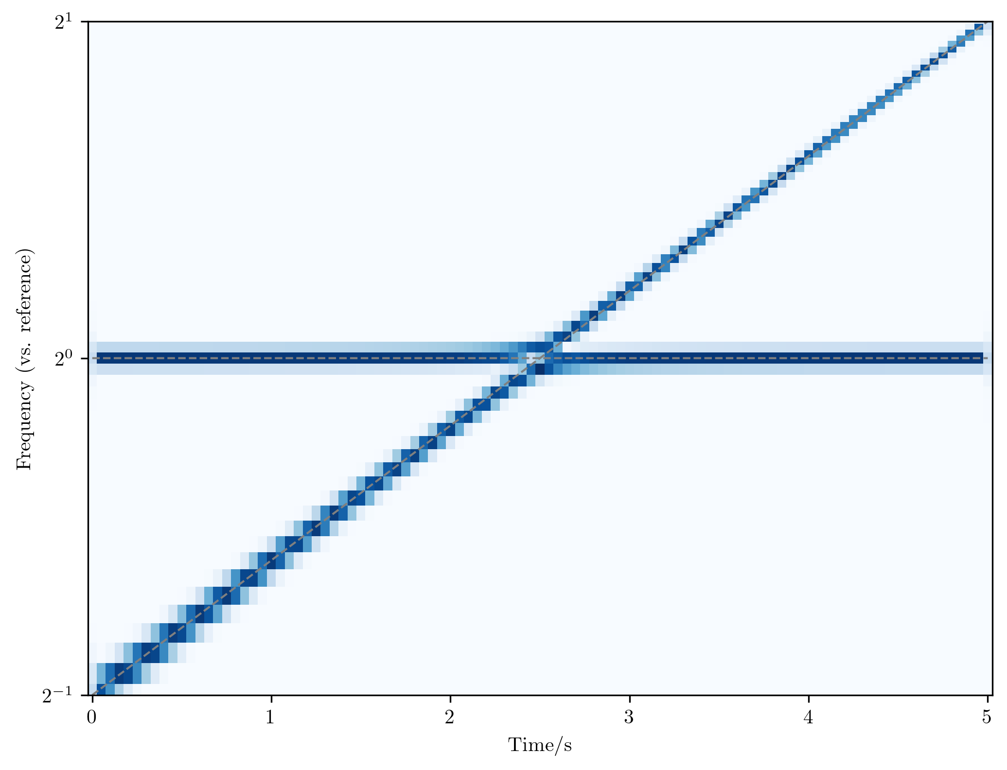
For very weak coupling ($\alpha \lesssim 10\ \mathrm{Hz}$) it's debatable whether we can hear any difference at all. The avoided crossing also can't be easily made out on a spectrogram. Here is $\alpha = 4\ \mathrm{Hz}$:

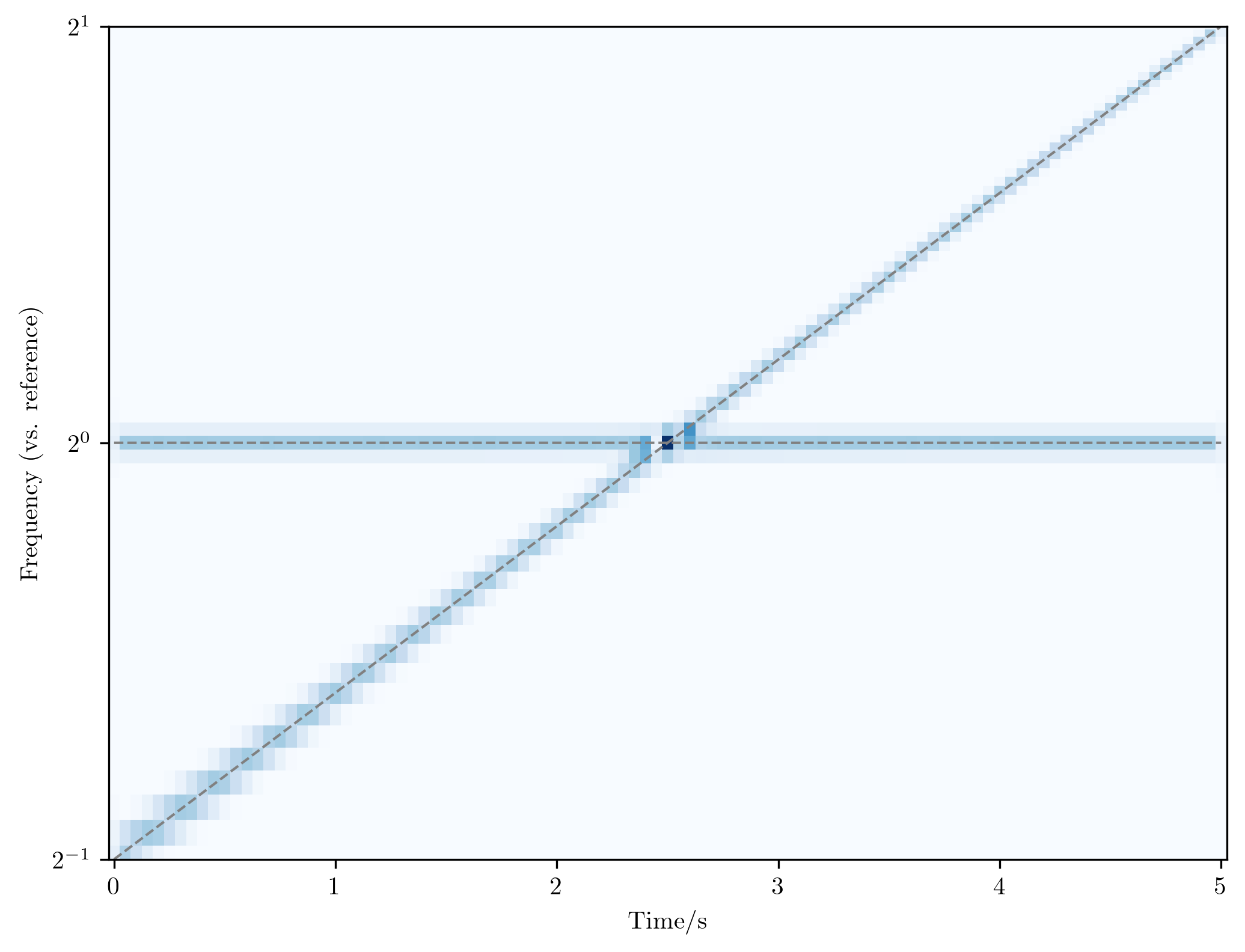
And here is $\alpha = 9\ \mathrm{Hz}$:

Intermediate Coupling

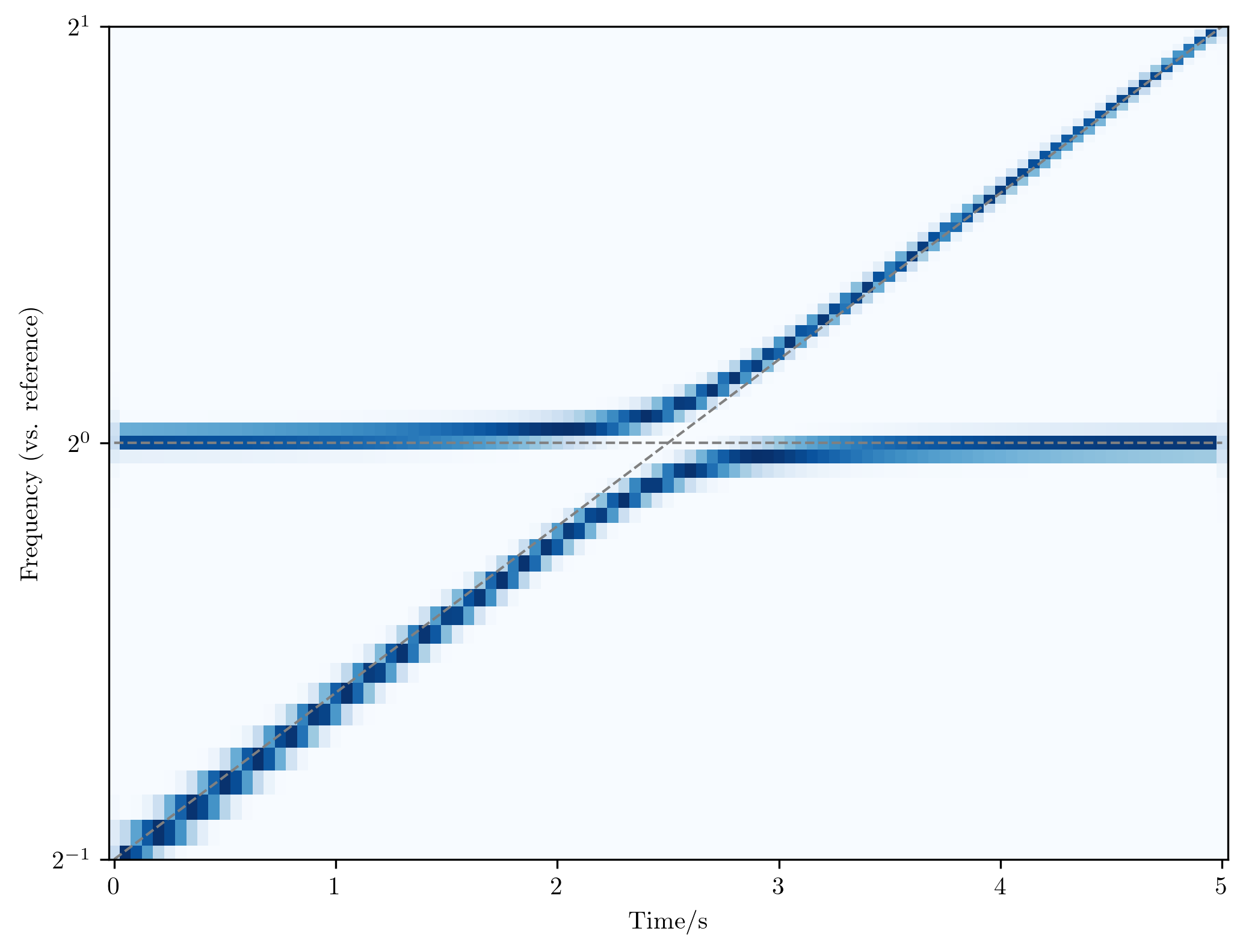
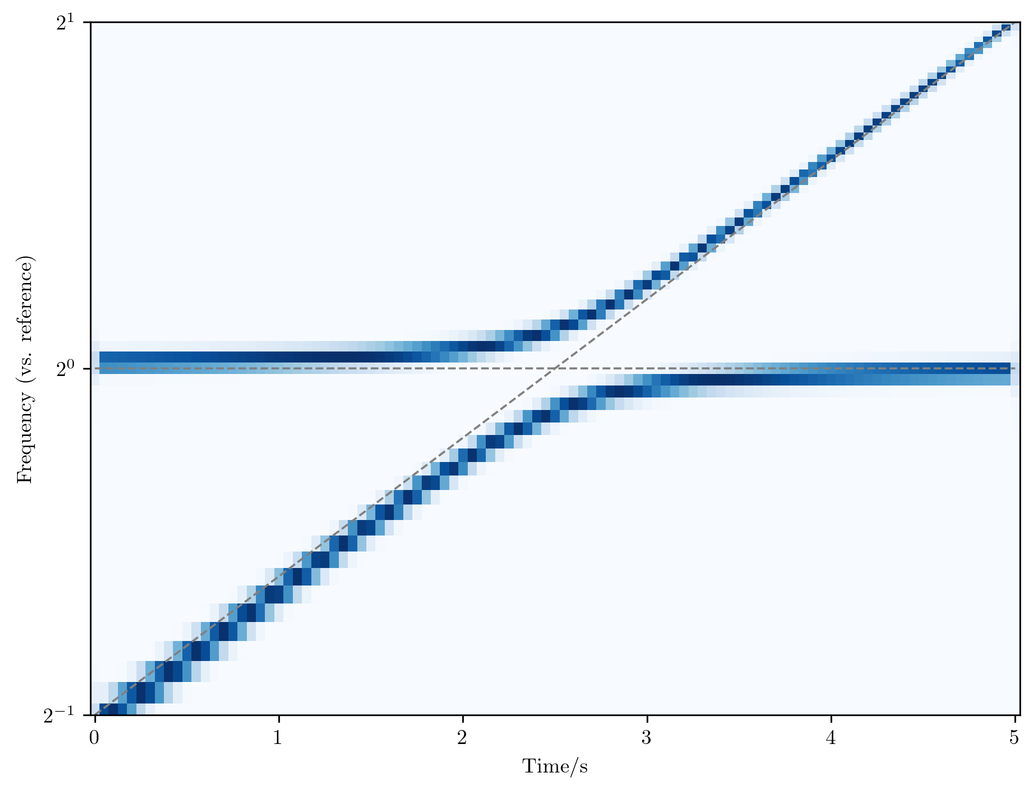
At $\alpha \sim 15\ \mathrm{Hz}$ the avoided crossing becomes visually apparent. Is it just me, or can I hear a real difference now?

As we keep increasing the coupling strength, the deviation from the pure configuration becomes more and more obvious.

Strong Coupling

For very large coupling, the frequency sweep we're using isn't wide enough, and so there's nontrivial mixing even at the beginning and end of our time interval covering the intersection: we're not able to hear the original pure tone and sweep.

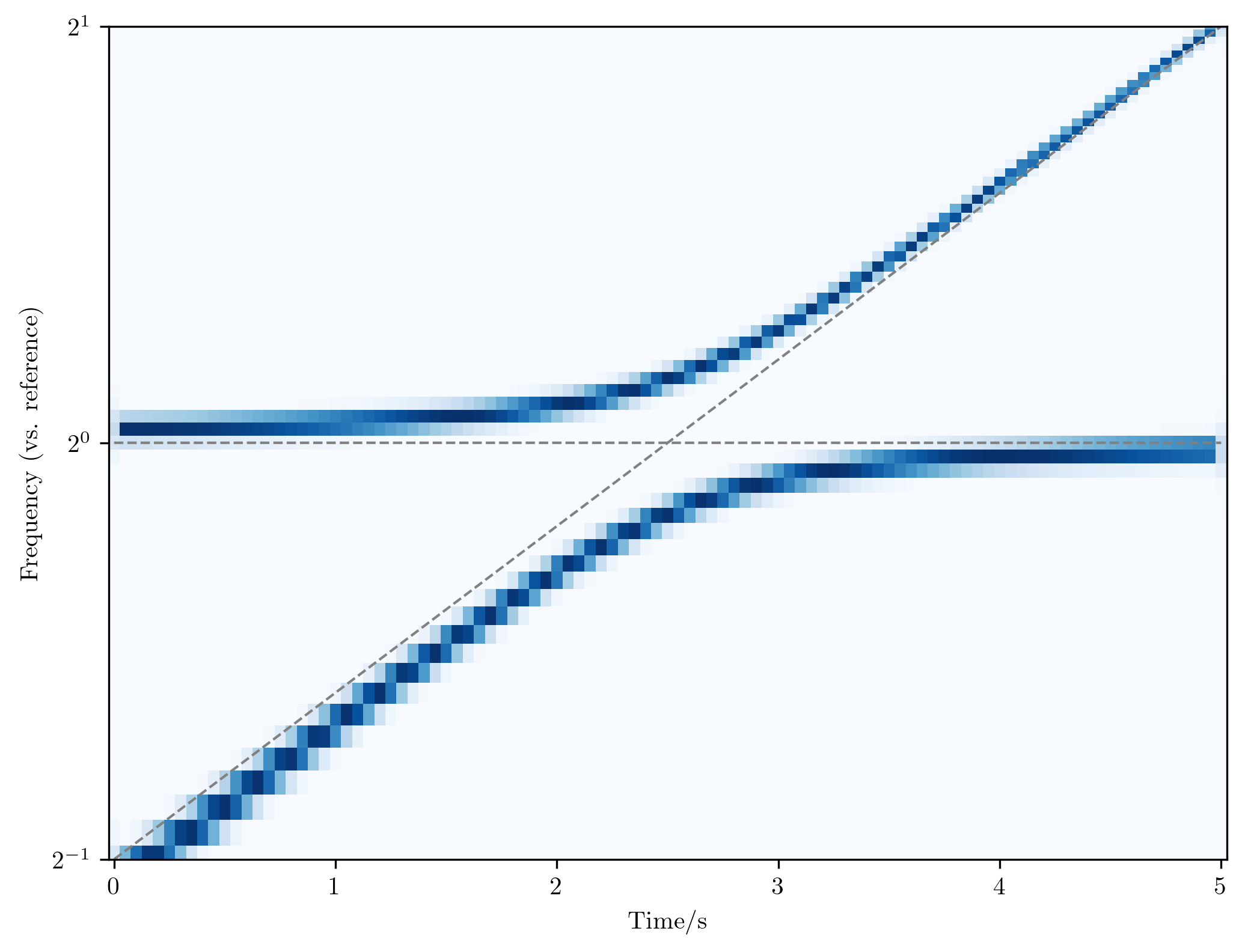
So yes, you can hear an avoided crossing! I don't really know how to articulate a good description of what I'm hearing, but at the very least I now have a rough idea of what to look out for qualitatively if I should wish to identify avoided crossings in nature by hearing alone. I hope you, the reader, found this as educational as I did.